


An easy way to improve quality
Many organisations today recognise that software development is so important that it requires a commitment to continuous process improvement.
Periodic assessments of "capability" are used both as a benchmark to confirm competitive position and as a marketing tool. But such assessments are essentially qualitative; there is a significant body of evidence that such capability assessments do, in fact, also correlate with quantitative measures of productivity and quality.
Quantitative measurement of software development is a very powerful management technique although "metrics" is sometimes seen as a difficult subject and can be misleading or mis-used.
Quantitative analysis, however, can teach us some important insights. In particular there is one factor, quite independent of capability, which has a major impact on the cost and quality of projects - and that is time pressure.
The management response to aggressive deadlines is frequently to throw staff at a project in the hope that it will speed up delivery. In many situations it is true that additional staff will save development time, although clearly there comes a limit beyond which it is not practical.
Equally of course - and this is not often considered - team size can be reduced, resulting in longer schedules. This is usually seen as an unfortunate consequence of lack of staff (or the right skills), but we shall see that it is a very effective strategy for improving quality while, at the same time, reducing cost.
Quantitative methods depend on measurements from projects equations link those measurements and calculate performance parameters. Such equations should be derived from data from lots of projects and many such models exist.
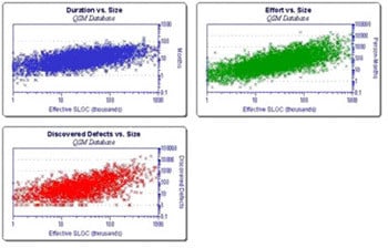
Raw data from many projects: duration, effort and defects are plotted against software size to reveal quantitative relationships.
Some mathematical models are complex, with lots of parameters, depending on lots of measurements for each project. Others are much simpler and this is generally an advantage.
Firstly simple models are easier to understand and explain to an audience (e.g. senior management). Secondly, because they are relatively simple, it is easy to vary parameters and explore alternatives; and thirdly, they are much easier to calibrate for a specific organization or environment than models which need lots of measurements.
One such model is the Rayleigh-curve model, developed by Larry Putnam from earlier work at IBM on hardware developments. Originally the model was used to estimate project cost and duration but it quickly became apparent that it could be extended to include software defects.
A Rayleigh curve is a good approximation to several aspects of software projects, for instance the size of the project team as it varies through the project lifecycle and also the rate of defect detection through the lifecycle.
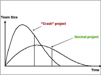
By changing parameters, many different curves can be generated, matching different size projects, teams, durations and quality. For staffing, the area under the curve is the total project effort; for defects, it is the total number of defects in the software.
One of the attractions of this particular model is that the equations generate two very useful parameters which directly relate to management.
One parameter quantifies "productivity" and the other indicates the "steepness" of the Rayleigh curve and can be thought of as a measure of time pressure. The outcome (i.e. the timescale, cost and quality) depends on both these parameters.
What’s the point of this? Well you can use a model like this in two ways. Firstly you can calibrate the performance of completed projects and measure the levels of productivity achieved. Secondly you can generate project estimates from assumptions about a new development.
Using the Rayleigh curve model, there are two parameters which are required as input to a project estimate: firstly it is necessary to express how big the proposed system is, and secondly it is necessary to express the level of capability (productivity) which can be expected in the development environment.
Of course there is usually significant uncertainty in both these assumptions but, quite reasonably, any estimate must itself be uncertain if you don't know quite what has to be developed and how it will be developed.
The Rayleigh model can quickly generate a range of estimates corresponding to a range of assumptions for both size and productivity. However there is a third parameter which the modeler can invoke - team size (or time pressure). By specifying a larger team, you can generate shorter schedules in your estimate but at rapidly increasing cost.
Project Estimates: Sensitivity Charts
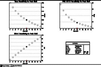
The charts above show how project estimates vary as the size of the team (measured at its peak size) is varied. The top left chart shows duration varying from 12 months down to just over 9 months as the team size increases from 4 staff to 15. The bottom left chart shows the corresponding cost in man months. It rises from an economic 33 man months to a costly 94 man months.
The top right chart shows the reliability of the software at delivery, measured as the Mean Time To Defect (MTTD). This is a direct reflection of the number of defects built into the software.
At a low team size, reliability is good, with an MTTD of almost 48 hours (one new bug in every 48 hours of operation). With a larger team of 15, the MTTD falls to about 12 hours - 4 times as many defects!
Reliability is rarely considered during the project estimation process but we can see that our planning assumptions have a major impact on it. And reliability, in turn, has a major impact on cost - the cost of bug-fixing after delivery and the cost of poor system performance whether in terms of disruption or customer relations.
The Rayleigh model we used above can be extended to look at the time and effort required after delivery – what does it take to achieve a specified level of reliability? By way of a benchmark, let's consider the estimate above based on a peak team of 4 staff.
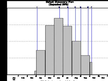
Defect discovery rate for a peak team size of 4
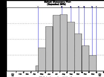
In the chart above, the project starts on Jan 1st and coding starts mid-April. By the time the project delivers, at the end of December, we are expecting less than 5 defects per month to be found corresponding to our MTTD of 48 hours.
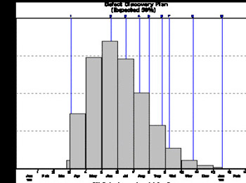
When we increase the team size to 15, coding (and defect detection) starts earlier and delivery is 2½ months earlier than with 4 staff. But the defect detection rate is only just under 20 bugs per month. Now lets us model an extension to the project to fix the outstanding bugs - perhaps a "warranty" phase.
We can see that reliability finally hits the "5 per month level" sometime in December. In terms of reliability, the 2½ month apparent saving is in fact less than one month. And the cost is, of course, even greater than the development cost because of the extra post-delivery bug fixing.
Only by collecting project metrics and analyzing them is it possible to understand these effects. But the practical and financial benefits of applying quantitative models are very great. It is possible to improve quality and save money at the same time!
Anthony Hemens, Managing Director of Quantitative Software Management (UK)